Quadtree in Particle Physics: A Computational Approach

Quadtree is a hierarchical data structure (tree) used to organize and divide a two-dimensional space into four smaller regions, called quadrants. This process occurs recursively: each internal node of the tree always branches into four children, while the leaf nodes represent the final regions, which do not need to be subdivided further. This structure is especially useful for efficiently storing, manipulating and searching spatial data.

The figure above shows a Point-Region quadtree, a structure that partitions space based on specific points. Quadtrees can be classified according to the data they represent. Among the most common types, the following stand out:
- Point-Region: Focuses on dividing space based on individual points, ideal for mapping georeferenced locations or events.
- Region: Divides continuous areas, being useful in analyses of land occupation or temperature variations.
- Edges: Represent contours and linear shapes, used to model road maps or borders.
- Polygonal Map: Stores polygons and their spatial relationships, applicable in cartography and geographic information systems (GIS).
- Compressed: Groups homogeneous regions to optimize storage, useful for compressing images and graphics.
In this article, the focus will be on the Point-region type, explaining its operation and practical applications.
How does the Point-Region Quadtree work?
A point-region quadtree is a structure that organizes two-dimensional space. Regions are recursively divided into four equal quadrants. Each region (or node) stores specific points within a delimited area. When the maximum capacity of a node is reached, it is subdivided into four new child nodes: Northwest (NW), Northeast (NE), Southwest (SW) and Southeast (SE). This subdivision process continues until the nodes no longer need to be divided, forming the so-called leaf node.
Node structure.
The node structure is similar to that of a binary tree, but with four pointers (children) instead of two. In addition, nodes contain essential information for locating points in space:
- Four pointers: Correspond to the quadrants North West (NW), North East (NE), South West (SW) and South East (SE).
- Point: The position of the stored point.
- Key: The x and y coordinates of the point.
- Value: Metadata or any information associated with the point.
This structure is widely used in systems that handle large volumes of spatial data, such as interactive maps, navigation systems, and georeferenced databases. The simplicity and efficiency of the point-region quadtree make it a very good choice for storing and retrieving spatial information quickly and in an organized way.
Practical applications
| Application | Description |
|---|---|
| Computer graphics | Used in image compression, vector graphics storage and fractal representation. |
| Spatial indexing | Store and query geographic maps and terrain data efficiently. |
| Collision detection | Used in video games and physics engines for efficient object interaction calculations. |
| Image processing | Image segmentation, region-based image compression and quadrant-based ray tracing. |
| Machine Learning | Accelerating nearest neighbor searches in KNN algorithms. |
Time complexity
| Operation | Complexity |
|---|---|
| Insert | \(O(\log{n})\) to \(O(no)\) (depends on balancing and distribution) |
| Search | \(O(\log_{n})\) (for well balanced trees) |
| Remover | \(O(\log_{n})\) to \(O(n)\) (may require merging nodes) |
| Range query | \(O(\ k \ + \ log_{n})\) to \(O(n)\) (where \(K\) is the number of elements returned) |
Quadtree and Physics: Robbie's Challenge
In the high-energy physics lab, Robbie, our curious robot, works with a team of scientists to unravel the mysteries of the universe. During an experiment, Gloria, one of the renowned physicists involved in the research, entrusts Robbie with the task of analyzing the collected samples. She asks him to identify, among the thousands of “hits” - the interaction points where particles emerge after intense collisions - the regions of greatest concentration and calculate the average electrical charge released in these events. Robbie, eager to learn more about the world of particle physics, accepts the challenge and begins working on his code.
note: In this article, we use the dataset from the TrackFormers - Collision Event Data Sets experiment. The data has 3 dimensions (x, y, z), but to simplify the explanation, we consider only the x and y dimensions. It is worth noting that, for three-dimensional data, the most appropriate structure would be an Octree
To simplify understanding, we implemented the examples in Python. However, the repository also contains Quadtree implementations in C# and Rust. You can access the complete code in the GitHub repository: .
Load detected particle collisions
Download the dataset
    import requests
    import tarfile
    import os

    dataset_url = 'https://zenodo.org/records/14386134/files/trackml_40k-events-10-to-50-tracks.tar.gz?download=1'
    local_tar_path = 'datasets/trackml_40k-events-10-to-50-tracks.tar.gz'
    local_extract_path = 'datasets/trackml_40k-events-10-to-50-tracks'

    if not os.path.exists('datasets'):
        os.makedirs('datasets')

    if not os.path.exists(local_tar_path):
        print('Downloading dataset...')
        with open(local_tar_path, 'wb') as f:
            response = requests.get(dataset_url, stream=True)
            for data in response.iter_content(chunk_size=1024):
                if data:
                    f.write(data)

        print('Extracting dataset...')
        with tarfile.open(local_tar_path) as tar:
            tar.extractall(local_extract_path)

    print('Dataset ready!')
    Downloading dataset...
    Extracting dataset...
    Dataset ready!
Load the dataset
    import pandas as pd
    from IPython.display import display

    path = 'datasets/trackml_40k-events-10-to-50-tracks/trackml_40k-events-10-to-50-tracks.csv'
    df_collisions = pd.read_csv(path)[['x', 'y', 'q', 'particle_id']]
    display(df_collisions.head(10))

    print(f'Total of detected particle collisions: {len(df_collisions)}')
Total of detected particle collisions: 9949945
Result of df_collisions

Extract and view samples for analysis
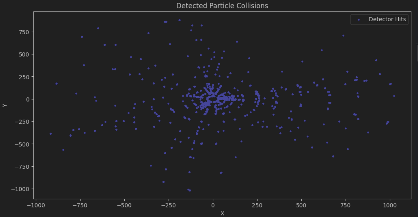
To simplify the analysis, Robbie decides to take a random sample of 2000 collisions.
    from helper import visualize_samples
    df_samples = df_collisions[0:2000]
    visualize_samples(df_samples)
Create clusters from detected particle collisions
Create two-dimensional space
Robbie needs to create a two-dimensional space to represent the detected particle collisions. He starts by converting each collision into a point in space, where the x and y coordinates represent the position of the collision in the detector.
Implementation of the Point class to represent points in space.
    from dataclasses import dataclass
    @dataclass(slots=True)
    class Point:
        x: int
        y: int
        metadata: dict = None

        def __repr__(self):
            return f'Point({self.x}, {self.y})'

    points = [Point(row.x, row.y, metadata=row.to_dict()) for index, row in df_samples.iterrows()]
    points[:10]
    [Point(-57.419, -67.1905),
    Point(-49.4727, -58.4256),
    Point(-41.6409, -49.6406),
    Point(-36.2328, -43.3855),
    Point(-36.4109, -43.582),
    Point(-31.0184, -37.3745),
    Point(-30.8612, -37.1731),
    Point(-30.9992, -37.3324),
    Point(-26.4289, -32.0082),
    Point(-26.2202, -31.8162)]
Implementation of the Rectangle class to represent regions in space.
@dataclass(slots=True)
class Rectangle:
    x: int
    y: int
    width: int
    height: int

    def contains(self, point):
        return (self.x <= point.x < self.x + self.width and
                self.y <= point.y < self.y + self.height)

    def intersects(self, other) -> bool:
        return not (other.x > self.x + self.width or
                other.x + other.width < self.x or
                other.y > self.y + self.height or
                other.y + other.height < self.y)

    def __repr__(self):
        return f'Rectangle({self.x}, {self.y}, {self.width}, {self.height})'
To create the two-dimensional space with the correct dimensions, Robbie decides to use the bounding box technique, which is a rectangular box that encloses all the points. He implements the function compute_bounding_box that calculates the bounding box from a list of points.
    def compute_bounding_box(points: list) -> Rectangle:
        min_x = min(p.x for p in points)
        max_x = max(p.x for p in points)
        min_y = min(p.y for p in points)
        max_y = max(p.y for p in points)
        return Rectangle(min_x, min_y, max_x - min_x, max_y - min_y)

    boundary = compute_bounding_box(points)
    boundary
Rectangle(-916.693, -1016.22, 1939.953, 1897.181)
Quadtree Implementation
Robbie starts implementing the Quadtree structure, he defines the Quadtree class with the boundary and capacity attributes.
    import numpy as np

    class Quadtree:
        def __init__(self, boundary: Rectangle, capacity):
            self.boundary = boundary
            self._capacity = capacity
            self.points = np.empty((capacity, 2), dtype=np.int32)
            self._metadata = np.empty(capacity, dtype=object)
            self._point_count = 0
            self._divided = False

            self._north_east = None
            self._north_west = None
            self._south_east = None
            self._south_west = None

        def subdivide(self):
            x = self.boundary.x
            y = self.boundary.y
            w = self.boundary.width
            h = self.boundary.height

            half_width = w // 2
            half_height = h // 2

            # Create four children that divide the current region
            nw = Rectangle(x, y, half_width, half_height)
            self._north_west = Quadtree(nw, self._capacity)

            ne = Rectangle(x + half_width, y - half_height, half_width, half_height)
            self._north_east = Quadtree(ne, self._capacity)

            sw = Rectangle(x, y + half_height, half_width, half_height)
            self._south_west = Quadtree(sw, self._capacity)

            se = Rectangle(x + half_width, y + half_height, half_width, half_height)
            self._south_east = Quadtree(se, self._capacity)

            # Mark the current region as divided
            self._divided = True

        def insert(self, point: Point):
            if not self.boundary.contains(point):
                return False # Point is not in the boundary

            # If there is space in the current region
            if self._point_count < self._capacity: #
                self.points[self._point_count] = (point.x, point.y)
                self._metadata[self._point_count] = point.metadata
                self._point_count += 1
                return True

            # If there is no space and the region is not divided
            if not self._divided:
                self.subdivide() # Subdivide the region if it hasn't been divided yet

            # Try to insert the point into the children regions
            return (self._north_west.insert(point) or
                    self._north_east.insert(point) or
                    self._south_west.insert(point) or
                    self._south_east.insert(point))

        def insert_batch(self, points: list):
            for point in points:
                self.insert(point)

        def query(self, boundary: Rectangle, found=None):
            if found is None:
                found = []

            # Return if the range does not intersect the boundary
            if not self.boundary.intersects(boundary):
                return found

            for i in range(self._point_count):
                point = Point(*self.points[i], metadata=self._metadata[i])
                if boundary.contains(point):
                    found.append(point)

            if self._divided:
                self._north_west.query(boundary, found)
                self._north_east.query(boundary, found)
                self._south_west.query(boundary, found)
                self._south_east.query(boundary, found)

            return found
Explanation of implementation
In the class constructor, we define:
- boundary: An object of type
Rectanglethat delimits the region of the node. - points: A pre-allocated NumPy array to store the coordinates of the points, with dimension
(capacity, 2). - _capacity: Maximum number of points the node can store.
- _metadata: An array to store the metadata associated with each point.
- _point_count: Counter of points entered.
- _divide: Flag indicating whether the node has already been subdivided.
- _north_east, _north_west, _south_east, _south_west: Child nodes representing the quadrants of the region.
Method subdivide()
When the number of points reaches its maximum capacity, the subdivide method is called. It calculates half the width and height of the current region and creates four new child nodes, each covering a portion of the original rectangle. This division allows points to be distributed into smaller regions, making future queries easier.
Method insert()
The insert method adds a new point to the Quadtree:
- Checks if the point is within the boundary region of the current node.
- If there is space on the node (i.e. point_count < capacity), the point and its metadata are added.
- If there is no space and the region has not been divided, the region is subdivided.
- If the region has been split, the point is inserted into one of the child nodes.
The insert_batch method allows you to insert multiple points at once.
Method query()
The query method performs a search for points that are within a rectangle (the query region).
- Checks whether the query region intersects the current node's region.
- If there is intersection, check whether the points of the current node are within the query region.
- If the region has been split, the search is performed on the child nodes.
The result is a list of points (reconstructed with their metadata) that satisfy the query condition.
Analyze particle collisions
With the Quadtree implemented, Robbie can start analyzing particle collisions. He creates a Quadtree with the bounding box of the two-dimensional space and inserts the detected collisions.
    quadtree = Quadtree(boundary, capacity=10)
    quadtree.insert_batch(points)
How to analyze regions automatically?
Robbie is faced with a challenge: how to automatically traverse each region of space to identify areas with the highest density of particle collisions? Performing this process manually, passing in the coordinates one by one, would be unfeasible, due to the vastness of space and the unpredictable distribution of regions of interest.
To solve this problem, Robbie decides to use a data processing technique that automates the analysis of different areas of space. He implements the SlidingWindowQuery class, which systematically scans the space, evaluating the density of collisions in each region. This approach allows him to identify patterns and critical areas efficiently and accurately.
    class SlidingWindowQuery:
        def __init__(self, quadtree: Quadtree):
            self._quadtree = quadtree

        def query(self, **kwargs):
            window_size = kwargs.get('window_size', 10)
            step_size = kwargs.get('step_size', window_size / 2)
            density_threshold = kwargs.get('density_threshold', 3)

            found = []
            boundary = self._quadtree.boundary

            x_start, y_start = boundary.x, boundary.y
            x_end, y_end = boundary.x + boundary.width, boundary.y + boundary.height

            x_values = np.arange(x_start, x_end - window_size + step_size, step_size)
            y_values = np.arange(y_start, y_end - window_size + step_size, step_size)

            for x in x_values:
                for y in y_values:
                    window = Rectangle(x, y, window_size, window_size)
                    points = self._quadtree.query(window)
                    if len(points) >= density_threshold:
                        found.append((window, len(points), points))

            return found
Explanation of implementation
The SlidingWindowQuery class performs a sliding window search on the quadtree, evaluating the collision density in each region.
- Query Parameter
Thequerymethod accepts three parameters:- window_size: Size of the search window.
- step_size: How much the window moves each iteration.
- density threshold: Minimum number of points that the window must contain to be considered relevant.
- Defining the Search Space:
The code uses the quadtree's boundary to know the total space to be analyzed and calculates the start and end points for the windows. - Window Movement:
With
np.arange, a series of values is generated for the x and y coordinates, allowing the window to span the entire space. - Checking in Each Window:
For each position, a window (a rectangle) is created and the quadtree is queried to find the points within that window. If the number of points is equal to or greater than the
density_threshold, that window is recorded as an area of interest. - Result: At the end, the method returns a list with the relevant windows, along with the point count and the points found themselves.
With everything ready, Robbie can now analyze the regions of highest density of particle collisions.
    window_size = 100 # Size of the window to analyze
    step_size = 25 # Step size to slide the window
    density_threshold = 20 # Minimum number of collisions in the window

    sliding_window_query = SlidingWindowQuery(quadtree)
    query_result = sliding_window_query.query(window_size=window_size,
                                              step_size=step_size,
                                              density_threshold=density_threshold)
    display(query_result[:1])
    [(Rectangle(-841.693, -416.22, 100, 100),
    20,
    [Point(-788, -343),
    Point(-757, -336),
    Point(-804, -405),
    Point(-804, -405),
    Point(-788, -343),
    Point(-757, -336),
    Point(-804, -405),
    Point(-804, -405),
    Point(-788, -343),
    Point(-757, -336),
    Point(-804, -405),
    Point(-804, -405),
    Point(-804, -405),
    Point(-804, -405),
    Point(-804, -405),
    Point(-804, -405),
    Point(-788, -343),
    Point(-757, -336),
    Point(-788, -343),
    Point(-757, -336)])]
View results
    from src.visualization import visualize_windows_results
    visualize_windows_results(quadtree, points, query_result)
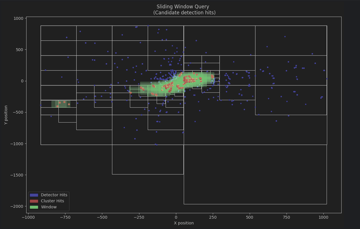
In the graph, the areas are subdivided by the quadtree into rectangles, representing the spatial organization that facilitates the localized analysis of collisions. The green area symbolizes the sliding window, which systematically scans the space, analyzing each sector in search of collision concentrations.
Blue dots mark detected events (Detector Hits), while red dots indicate areas with high collision density (Cluster Hits), highlighting clusters where multiple impacts occurred. Regions with a higher concentration of red dots represent areas of interest for analysis, highlighting significant collision patterns. The sliding scan, combined with the hierarchical structure of the quadtree, allows for efficient analysis, focusing directly on areas with the highest activity, while optimizing performance by avoiding unnecessary scans in low-density regions. This approach combines accuracy and efficiency to reveal spatial patterns of collisions.
Analyzing the clusters
    clusters = []
    for window, count, cluster_hits in query_result:
        cluster = {
            'coordinates': (window.x, window.y),
            'particles_count': count,
            'avg_particle_charge': np.mean([point.metadata['q'] for point in cluster_hits]),
            'particles': [point.metadata for point in cluster_hits]
        }
        clusters.append(cluster)

    display(pd.DataFrame(clusters))
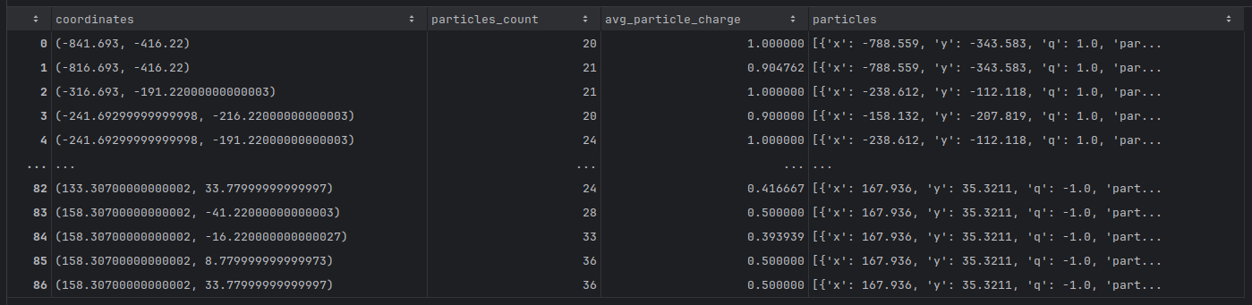
Robbie looks at the cluster data and analyzes the table he obtained. This table presents the results of the automatic scan he implemented, highlighting the main metrics for each region examined.
Robbie's first observations are in the coordinates column, which shows the central coordinates of each area analyzed, indicating the specific points in space where collisions occurred. He then analyzes the particles_count column, which reveals the total number of particles detected per region. By noticing significant variations in this number, Robbie identifies areas of higher density, which may indicate regions of interest for his study.
Robbie looks closely at the avg_particle_charge column, which displays the average electrical charge of the detected particles. He notices that values close to 1.0 indicate a predominance of positive particles, while negative or fractional values suggest a mixed distribution or a predominance of negative particles.
Finally, Robbie delves into the particles column, which contains a detailed list of detected particles, along with their coordinates and electrical charges (q). This granular view allows him to identify patterns, such as clusters of particles with similar characteristics, helping him better understand areas of high activity in the experiment.
With this analysis, Robbie presents the results to Gloria. She is impressed by the efficiency of the algorithm and the quality of the information obtained. With this data in hand, the team of scientists can now investigate the regions of highest collision density and identify patterns and trends in the data. This could lead to significant discoveries that will help unravel the mysteries of the universe.
Conclusion
The point-region quadtree is a powerful framework for organizing and analyzing spatial data. Its application in the study of particle collisions has demonstrated its effectiveness in identifying patterns and hotspots. With the help of the quadtree, Robbie and his team of scientists were able to explore large volumes of data quickly and accurately, reaffirming the importance of this framework for complex problems in science and technology.
References
- U. Odyurt e N. Dobreva. “TrackFormers - Collision Event Data Sets”. Zenodo, 2024. Link to article
- Wikipedia contributors. “Quadtree.”, 2025. Wikipedia, The Free Encyclopedia, 2025 Link to article